Nexus
is a student software project to be carried out in the University of Jyväskylä
during the spring 2002. The project implements a system of a distributed
computational Grid for VTT Information Technology. The system will make use of
Grid technology by using Globus Toolkit available freely from the Globus
organization.
The software project will collect information about
distribution and explore when it is efficient to use decentralization in
computational tasks. The practical software to be developed will calculate and
visualize three-dimensional fractals using distributed computing. A monitor for
analyzing the computational results with different sets of computers and data
amounts will also be made.
The software contains two
separate components. The client part includes the user interface and the
fractal visualization. From the end-user point of view, the application will
render fractal under consideration on a screen. The user can rotate it or zoom
the view and the fractal is then recalculated. The fractal calculation is
divided in specified amount of smaller tasks and then shared with several computers
connected as a network with Globus framework. The results are sent back to the
client machine as the calculation is going on.
This document describes how
the software will be implemented. Chapter 2 represents the goals and Chapter 3
the requirements of the software. In Chapter 4 the structure of a distributed system
is introduced. Chapter 5 describes the classes of the JavaCoG that are used in
the application and also shows the class diagram. The fractal calculation is
represented in Chapter 6 and the next chapter describes how the 3D
visualization of the fractals will be done. Chapters 8 and 9 describe the user
interface of the application and the use cases in connection with the user
interface. Chapter 10 represents the comments and the coding practices that are
used and Chapter 11 introduces the main features of the testing principles.
The goal of the project is to produce
information about the efficiency of distribution when the Globus toolkit is
used with different amounts of calculation tasks. The most important priority
is to implement a computational Java software which uses Globus toolkit in
distribution and operates on Windows 2000. It is also important to gather
information about the traffic in the network. It must be possible both to
control the calculation and to distribute it in several Linux computers by
using Globus and to calculate it just in the local machine. By enabling this,
it is possible to estimate the efficiency of the distribution. The secondary goals
include visualizing the calculation results impressively.
To achieve these goals, it
has been decided to implement a program that calculates and visualizes
3-dimensional fractals. The fractals are three-dimensional intersections of the
quaternion Julian sets. The program should cope with 1 to n fractals and the
calculation of each fractal can be distributed from 1 to n machines. The
decision has been made that it is enough if the program copes with nine
fractals. The aim of the distribution is that the calculation on each machine
is approximately equally demanding. The software should include functionalities
to determine the calculated area, the number of iterations and the rotation
angle for the fractals.
Because the application is
developed for gathering and presenting information on a limited area, the
graphical user interface, its usability and the functions are not the primary
things in this project. Instead, it is emphasized to produce accurate and
systematic measuring information about the distribution. In general, the
biggest part of efforts will be directed to handling the Globus and
distribution.
This
chapter clarifies the requirements of the software, user interface and
testing.
The
requirements for the software are listed below.
- The software must be able to
calculate 3D fractals with different number of iterations.
- The fractal calculation must be
distributable.
- It must be able to calculate
the fractals also in the same Windows 2000 machine where the user
interface is.
- Fractals must be able to be
zoomed i.e. to be calculated from different areas.
- Fractals must be able to be
rotated.
- A separate sniffer software
must be able to collect information about the network performance including
latency and bandwidth.
- The distribution is implemented
with the help of the Globus toolkit.
- The Globus toolkit is used
through the Java CoG library.
The user interface must operate on Windows 2000 and from there the user
must be able to
- view the fractals that are
under calculation or have been calculated,
- choose the number of iterations
of the fractal calculation,
- choose the machines that will
participate in calculating of each fractal,
- view the desired information about
the network performance and
- read
the log information from the machines that participate in calculating.
The
requirements for the software are the following ones:
- It must be tested that all the
requirements in Chapters 3.1 and 3.2 are working.
- The calculation must be tested
on one machine and on the different number of machines.
- The distribution results must
be compared.
- The conclusions must be
visualized.
A separate
measuring plan will be written that describes the requirements for testing more
specific.
This chapter describes the
structure of the system from the Globus point of view. The main features of it
can be seen in the Figure 1.
A Globus application
consists of the following components: a client application, broker, information
service, co-allocator and one or more GRAM components. Information between
these components is transmitted using the resource specification language
(RSL).
The information service provides access to information about the current
availability and capability of resources the user has access to. In the Globus
system the Metacomputing Directory Service (MDS) is used for maintaining
information service. MDS uses the data representation and the application
programming interface defined in the Lightweight Directory Access Protocol
(LDAP).
Resource brokers are responsible for taking RSL specifications and
transforming them into more concrete specifications. These can be passed for
example to a co-allocator that is responsible for coordinating the
allocation and management of resources at multirequests. Co-allocator splits
the request into its components, submits each component to the appropriate
resource manager and handles the resulting set of resources as one. Dynamically
Updated Request Online Co-allocator (DUROC) is a component for handling all
these tasks.
GRAM (Globus Resource Allocation Manager) belongs to the
lowest level of the resource management architecture in the Grid technology. It
is responsible for processing RSL specifications representing resource requests
by either denying the request or by creating one or more processes according to
the request. It also enables remote monitoring and management of the created
jobs and updates the MDS information service with information about the current
availability and capabilities of its resources.
The principal components of
GRAM are the gatekeeper, the job manager, the local resource manager, the RSL
parsing library and the MDS: Grid Resource Information Service. The GSI (Globus
Security Infrastructure) is used for authentication.
The task of the gatekeeper
is to respond to requests of other machines. This is done by doing three
things: performing mutual authentication of user and resource, determining a
local user name for the remote user and starting a job manager which is
executed as that local user and actually handles the request. The first two
tasks are performed by calls to the GSI.
A job manager creates
the actual processes the user has requested with help of the RSL Library. This
usually involves submitting a resource allocation request to the underlying
resource management system. The job manager handles the monitoring of the state
of the created processes. It also notifies the callback contact if the state of
the process changes and implements control operations such as process
termination.
The MDS: Grid Resource
Information Service is responsible for storing into MDS various information
about scheduler structure and state. This includes e.g. total number of nodes,
number of nodes currently available, currently active jobs and an expected wait
time in a queue.
Figure
1. The structure of the Globus system in the
project.
In this
chapter the classes that will be used to implement a distributional software
are described. Most of them are part of the Java CoG library but a few classes
have to be implemented. All these classes can be seen in the class diagram in
Figure 2.
The
application has the class GlobusClient that controls the usage of the Globus toolkit. It implements the
interface GramJobListener. The class JobListener implements the interface JobOutputListener and handles the output of the GramJobs.
The class GlobusClient uses the class org.globus.mds.MDS to get information of available
resources and collects the information to hashtable mdsResult. After locating the resources the
class GlobusClient uses the class org.globus.gram.Gram to ping the computers meant to use.
Then the class GlobusClient creates a new gramJob using the class org.globus.gram.GramJob and adds it to the gramJobList.
To create GramJob the class GlobusProxy and the string rsl are needed. The class GlobusProxy contains the user key and the user
certificate of the globus. The string rsl is created by using the class org.globus.gram.GramAttributes.
When all
the initializations above have been made the gramJobs are transmitted to the resources
(GRAM) by using the method request of the class org.globus.gram.GRAM. When the status of each job
changes the method statusChanged in the class GlobusClient is called.
Each output
of the gramJobs goes to a different output file to the
computer where GASS server is located. The class GassServer redirects each output file to the
separate jobOutputStream stream. When output of each jobOutputStream is updated the method outputChanged in the class GlobusClient is called. When GramJob is finished and no more output is
generated method OutputClosed in the class GlobusClient is called.
The classes
below will be developed for the distribution.
The class GlobusClient implements GramJobListener.
The class manages the use of the Globus toolkit, listens to the state changes
of the GramJobs and commands the visualization class to draw
given pixels. The attributes of the class are listed below.
Vector gramJobList is a list of all
existing GramJobs.
HashTable mdsResult is a hashtable that contains the results of mds
searches.
The methods
of the class are listed below.
public
statusChanged()is used to notify the implementer when the status
of a GramJob
has changed.
The class JobListener implements JobOutputListener.
It handles the outputs of GramJobs. The methods of the class are
listed below.
public
outputChanged(java.lang.String output) is called whenever the
job's output has been updated.
public
outputClosed() is called
whenever job is finished and no more output will be generated.
The classes
below from the package org.globus will be used for the distribution.
The class org.globus.gram.Gram
has the constructor Gram().
Methods of the class are listed below.
request(String
resourceManagerContact, GramJob job) is used to transmit a GramJob
to the specific Gram.
cancel(GramJob
job) cancels a GramJob.
ping(GlobusProxy
proxy, String resourceManagerContact)pings the resource manager
The class org.globus.mds.MDS has the constructor MDS(String hostname, String
port). The
methods of the class are listed below.
connect() connects to the
specified server.
disconnect() disconnects from
the MDS server.
Hashtable search(String baseDN, String
filter, String[] attributes int searchScope) issues a
specified search to the MDS.
The class org.globus.io.gass.server.GassServer
has the constructor GassServer(GlobusProxy proxy, int port). The
methods of the class are listed below.
OutputStream getOutputStream(String id) returns the
output stream of the GassServer.
registerJobOutputStream(String lb,
java.io.OutputStream out) registers the output file to the output stream.
The class
org.globus.io.gass.server.JobOutputStream has
the constructor JobOutputStream(JobOutputListener jobListener). The
methods of the class are listed below.
close() notifies the jobOutputListener that no more
output will be produced.
The class org.globus.gram.GramJob has
the constructor GramJob(GlobusProxy proxy,
String rsl). The class has the following methods:
String getStatusAsString() returns the status
of the job as string.
cancel() cancels the job.
GlobusURL getID() returns the JobID as GlobusURL.
The class org.globus.security.Globus.Proxy has the constructor GlobusProxy(java.security.PrivateKey
key, java.security.cert.x509Certificate[] certs).
The class org.globus.gram.GramAttribute
has a constructor GramAttributes(). The class
contains the following methods:
String toRSL() converts GramAttributes to string.
The chapter
explains how the fractal calculation will be implemented.
The
fractal objects that will be used in our software are quaternion number Julia
sets. A quaternion number has 1 real and 3 imaginary parts, and it is often
marked as c = (a, bi, cj, dk). Quaternion Julia sets are defined
correspondingly to typical Julia sets, using quaternion numbers instead of
complex numbers.
Let us
define the quaternion Julia set with a quaternion constant c and quaternion
set:
Definition
1: A quaternion number z is inside of a
set if a sequence
z(0) = z
z(n) = z(n-1)^2 + c
converges.
Definition
2: A quaternion
number z is inside of a set if a sequence
z(0) = z
z(n) = z(n-1)^2 + z
converges.
The software
to be developed will contain a 3D visualization of a 4D quaternion fractal.
This can be done by simply keeping one of the dimensions constant.
A fractal
object is calculated to a form of a depth buffer (or z-buffer). The depth
buffer is a two dimensional array which have on each (x,y)-position a value of a top z-coordinate of an object in
that position. The depth buffer is then rendered on the screen somehow.
The
chapter describes the information that a fractal calculating program in our
software uses.
An area on
3D-space where a fractal is calculated is defined by a start point (start_x, start_y, start_z)
and an end point (end_x, end_y, end_z). Quaternion fractal objects are presented with double precision
and their values belong to [(-2.0, -2.0, -2.0), (+2.0, +2.0, +2.0)].
The number of the iterations (integer) defines how many times the sequence z(n)
= z(n-1)^2 + c is iterated until a decision can be made whether it is
converging or diverging. A bigger value means better estimation of a fractal
set but also longer computing time.
A Julia
quaternion constant C is defined as (C_x, C_y, C_z, C_w) which is represented with double
precision. In all interesting Julia-sets the values are small.
Rotation
angles are defined as (R_angle_x, R_angle_y, R_angle_z) and represented with integer values. They tell how many degrees
the object is rotated in x, y and z directions.
The number
of the steps in x, y and z direction (Steps_x, Steps_y, Steps_z) tells how many steps (integer)
the area is divided in calculation. Steps_x
and Steps_y determine how many x- and
y-elements the result depth buffer array contains eg. the resolution of an
image. They are typically set according to the resolution and the size of the
window that views the fractal.
Steps_z determine how smoothly the top z
value of a set in each (x,y)-position is searched. Bigger Steps_z means a smoother image but also a longer computing time.
Constant dimension value W
(double) is a value for dimension that is kept constant.
Let us
consider how the fractal computing will be implemented. The routines described
here might change a bit for a speed purpose.
The main
loop of a fractal calculator for one machine in a pseudo-code looks like this:
void Main (properties)
{
Origo = a middle point of an area defined by
(Start_x, Start_y, Start_z), (End_x, End_y, End_z)
for(Y_index = 0 to
Steps_y ) {
for (X_index = 0 to Steps_x) {
Z_index = 0;
Decision = false;
//depth_buffer element
is initialized with a value, which tells that there is no //object in this
position.
depth_buffer[X_index, Y_index] = -1;
//This
do-loop searches the top z-value by simply moving on z-direction one
//'Step_Z'
by one and testing on every point if it belongs to the fractal set.
//This
is very slow method and might have to be replaced because of a speed
//purpose.
(A split search would be much more efficient, but it doesn’t work /
//properly
in this case because the fractal-set is not "convex".)
do {
Value_X = ((End_x - Start_x) / Steps_X) * X_index;
Value_Y = ((End_y - Start_y) / Steps_X) * Y_index;
Value_Z
= ((End_z - Start_z) / Steps_X) *
Z_index;
Value_W = W; // constant dimension
//
Rotate value
(Value_X,
Value_Y, Value_Z) =
Rotate(Value_X,
Value_Y, Value_Z, R_angle, Origo);
// The value is inside a set.
Decision
=
Is_inside_a_set(Iterations,
Value_X, Value_Y, Value_Z, Value_W, C);
if (Decision == True) {
// Top Z-value was found and
is set in a depth_buffer.
depth_buffer[X_index, Y_index]
= Z_index / Z_Steps;
}
Z_index ++;
} while ((Z_index <= Steps_z) and (Decision = false))
}
}
}
The
subroutines simply rotate the point (x,y,z) around the given origo by the given
angles. This routine may have to be excluded because of speed purpose (rotating
will then be done on a main loop by moving on rotated base vector direction
beside of x-, y-, z-direction)
The
subroutine Is_inside_a_set estimates whether the value
belongs to Julia set. Its implementation looks like this:
Bool/int Is_inside_a_set(int Iterations, double x, y,
z, w, C_x, C_y, C_z, C_w)
{
Bool/Int decision;
Z = (x,y,z,w); // quaternion
int i = 0;
do {
Z
= Z^2 + C; // Julia
//
Z = Z^2 for quaternions is computed easily.
normp
= (Z.x)^2 + (Z.y)^2 + (Z.z)^2 + (Z.w)^2;
//
Vector's norm in the power of two.
i ++;
} while((i <= Iterations) and (normp <
4))
Decision = true;
// When the norm >=
2 the sequence diverges.
if (normp => 4) {
Decision = false;
}
return Decision;
}
We
distribute the fractal calculator described above to n different GRAMs
(machines) by creating n processes of a routine, each of one running under GRAM
of its own.
One of the
processes is a “master” process, which only collects the results of the fractal
calculation. Other processes are the “slave” processes that will do the
calculating work. The computing work is divided by letting each of the slave
processes compute their own part of horizontal lines of a depth buffer. Each
slave process can conclude it’s part by it's ID-number and the amount of
processes (these are given by MPICH-G2 and the master’s ID-number is zero).
Slave
processes send the calculating results to the master process by using MPI’s
message-passing routines. The master process then encodes the result depth
buffer line to the form of char. After this, it puts it in the output stream
from where the client Java-CoG program receives, decodes and finally draws it
in the screen.
The Main
loop then looks like this:
void Main (properties)
{
if MY_ID = 0 { // master process
while (calculating is going on) {
depthBuffer_line
= receive_data_from_the_slave_processes
encode(depthBuffer_line)
send_data_to_the_client(encoded_depthBuffer_line)
}
}
else { //
slave process
for (Y_value = MY_ID to Steps_y, by
step = Amount_of_Processes-1) {
//Mostly same as in
chapter 6.4, only depth-buffer-handling differs //since data is sended to the
master process one horizontal line by one.
send_a_data_the_master_process(depthBuffer_line);
}
}
So the
routine calculates horizontal lines of a depth buffer on every (Amount_of_Processes – 1) line starting from line MY_ID. This way every line will be calculated and the amount of
computing work is quite equal in each process.
The master
process will send the result data to the user interface by putting it in the
output stream. To do this, the integer depth data is encoded to the character
form. The integer contains 32 bits and character contains 8 bits, but in this
case the values are quite small (< 100000), so that only three characters
are needed in encoding one integer-value. Encoding is done by simply putting
the uppermost 8 bits of an integer value to the first character, the lower
8-bits to the second character, and the lowest 8 bits to the third character.
The line number of an encoded depth buffer line is put in the beginning of a
character table so that the client machine knows where to render the line in
the screen.
The
encoding of the integer value is done by the precision of three characters
(bytes):
Integer: aaaaaaaabbbbbbbbcccccccc
à Char 1 : aaaaaaaa Char 2 : bbbbbbbb
Char 3: cccccccc
After the
master process puts the encoded depth buffer line to the output stream, it will
be transferred to the machine that views the fractal by GASS server (this is
more precisely explained in Chapter 5.1).
The original requirements stated that the visualization should be
implement by Java 3D but there appeared a problem. Java 3D supports only
polygon rendering and not raster rendering, which is needed to visualize
complex images like quaternion fractals. Due to this we shall implement a small
rendering machine of our own by using standard Java packages.
The visualization contains two
parts. First there is a rendering part that takes a depth buffer of a fractal
object (see Chapter 6) and modifies it to the intensity buffer. Intensity buffer
is a two dimensional array which contains light intensity value for each (x,y)
pixel position. Secondly there is a drawing part that takes an intensity buffer
and modifies each brightness value to the RGB colour value, which is then
plotted to the corresponding (x,y) position in the screen. The depth buffer is
provided to the visualization part one horizontal line by one.
DB_Visualizer
is a class for visualizing the depth data computed by a fractal computing part
of the software. It contains its own viewing window and has a method for
visualizing the depth buffer horizontal line, which is given by one-dimensional
array and its y-position.
The class has attributes for a size
and resolution of a viewing window, for a size of a depth buffer array and
probably for some rendering information (colours, point of a light source
etc.). The class also needs the area from where the fractal is calculated
(start point and end point), the angles (angle x, angle y, angle z) that describe
how the fractal is rotated, and information about the resolution in x-, y- and
z-directions (first two describe the size of a depth buffer). It uses DB_Renderer class.
DB_Renderer
is a class for rendering the depth data. It transforms the pixel depth values
to the light intensity values in a way that result looks three-dimensional. It
contains attributes for a size of a depth buffer, for the area and rotating
angles of fractal, for the resolution in z-direction, as well as for some
information of rendering. It also contains brightness buffer array mentioned
earlier and a depth buffer array, which is needed in rendering.
The class contains a method for
rendering horizontal depth buffer line which is given by one-dimensional array
and its y-position. The given line is stored to the depth buffer array which
the intensity buffer array is used to be recalculate. There is a method for
getting data from the intensity buffer array, which is used by DB_Visualizer.
If the rendering method in DB_Renderer is implemented by ourselves, it
probably will be based on an idea of approximating the normal of the object’s
surface in each pixel point. The pixel point is here a point in 3d-space corresponding
to the pixel of a visualized object picture and to the position of a depth
buffer array. Approximation is done by using four or eight neighbouring pixel
points of a current pixel point. When the normal of the pixel point and the
point of the light source are known, the intensity of light for a pixel point (Ip)
can be calculated from the Lambert law:
Ip
= Il * Kd * cos A
In the formula Il is the
intensity of the light of the light source. Kd is constant between 0 and
1, which is an approximation to the “diffuse reflectivity”. In nature it
depends on the material of the surface and the wavelength of a light. A
is an angle between surface’s normal in the current point and the line
from the point to the light source. A varies between 0° – 90° (0 –
p/2), where the small
values represents high intensity of light (the surface is nearly towards to the
light source in the current point) while the big values represent low intensity
of a light. To make this calculating task easier, the light source might be set
to the infinity, which makes the line from the pixel point to the light source
to be a constant vector for every pixel point.
This
chapter describes the user interface and the dialogs and also shows the
pictures of them.
When the user starts the program there are only the command
menu File and few buttons in the top of the user interface (see Figure
3). In the same time the program starts, the MDS server is being contacted to
find out the resources on which the fractal calculation can be done. This
information is used when the user defines on which machines each of the
fractals will be calculated. In order to get new resources the user has to
apply for them directly from the owner of the wanted machines.
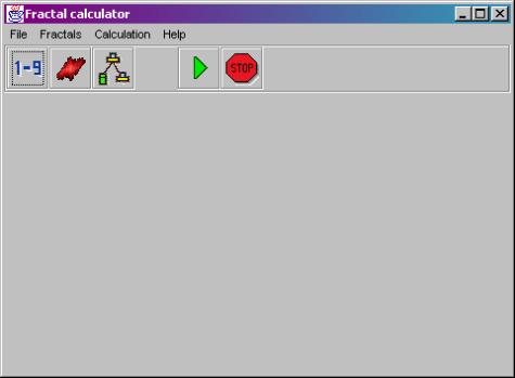
Figure
3. The main window of the user interface.
The user interface contains the command menus File,
Fractals, Calculation and Help. The first three buttons are
shortcuts choosing the number of calculating machines, the fractal parameters
and the calculating machines for each fractal. After all these values are
chosen the fractal calculation can be started either with the Start
button or from the Calculation menu. If the calculation is going on it
also can be cancelled before the calculation of the fractals is finalized. This
can be done with the Stop button or from the Calculation menu.
The number of calculated fractals can be chosen from the Number
of the fractals dialog seen in Figure 4. The user can choose from one to
nine fractals to be drawn.
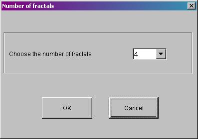
Figure
4. The number of the fractals dialog.
This dialog is meant for determining all the parameters in
connection with the calculation and the appearance of the fractals.
The values that affect to the calculation and the
visualization of the fractals can be determined from the dialog Fractal
Properties seen in Figure 5. The values in the first interleaf Shape
affect to the shape of the fractals. The values for the rotation angle, the
calculation area and Julia constant values can be determined.
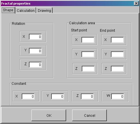
Figure
5. The parameter dialog for the shape of the
fractal.
The interleaf Calculation (Figure 6) contains the
values for determining how demanding the fractal calculation will be.
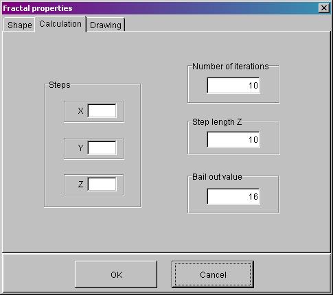
Figure
6. The parameter dialog for the fractal
calculation.
From the interleaf Drawing (Figure 7) the user can
determine the values attached to the drawing of the fractals. The color of the
fractals and the background, the coefficients affecting to the light as well as
the value for defining the roughness of the fractal surface can be determined.
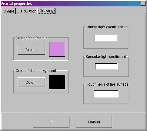
Figure
7. The parameter dialog for the visualization
of the fractals.
The dialog Calculating computers is seen in Figure 8.
In this dialog all the available machines for calculation are seen in the list
on the left side of the dialog. From these the user can determine the machines
on which the calculation of each fractal is distributed. The user can also
determine that the fractal calculation will be done on the local machine. This
can be done by choosing the item Calculate on this machine from the
bottom of the dialog.
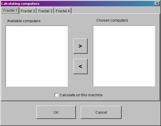
Figure
8. The dialog for choosing the calculating
machines for each fractal.
This chapter
describes the different use cases of the system.
Precondition: -
Description: The user starts the program.
Postcondition: The program has started. The default values
that define the fractal are set to the parameters. These values are the number
of the fractals and the fractal parameters. The calculating computers are
searched and they are shown in a list. The screen is empty.
Exceptions: There are no machines found or available at the
moment. The dialog that announces about the situation is shown.
Precondition: The program has started.
Description: The user chooses the command Number from the Fractals
menu. The program shows a dialog where the user can choose the number of the
fractals to be calculated. The number can be chosen between one and nine. The
number is accepted with the OK button and abandoned with Cancel
button.
Postcondition: The number that the user defined is set to the
variable and the dialog is closed.
Exceptions: -
Precondition: The program has started.
Description: The user chooses the command Properties from
the Fractals menu. After this the program shows a dialog with three
interleafs: Shape, Calculation and Drawing. From these the user
can determine values that define how demanding the calculation will be and how
the fractals will be visualized. These values are for example the number of
iterations, the rotation angle, the area from which the fractal is calculated
and the color of the fractal and the background. The options are accepted with
the OK button and abandoned with Cancel button.
Postcondition: The values are set to variables and the dialog is
closed.
Exceptions: The user inputs a number that is either too big or too
small. The value is not accepted and the default value is set to the text
field.
Precondition: There has to be machines available for the
calculation.
Description: The user defines the calculating machines for each
fractal from the dialog. In the dialog there is a list where all the available
machines are shown. The user can choose the calculating machines from this list
for every fractal. It is also possible to determine that the fractal will be
calculated on the local machine and not to be distributed. The choices are
accepted with the OK button and abandoned with the Cancel button.
Postcondition: The calculating machines are chosen and the dialog is
closed.
Exceptions: -
Precondition: The fractal parameters, the number of the fractals and
the calculating machines must be defined. There is no fractal
calculation going on.
Description: The user chooses the Start command from the Calculation
menu. After this the execution of the program propagates as described in
Chapters 6.5 and 6.6 with the parameters the user has defined. During the
calculation the results of it are transferred to the user interface machine
that visualizes the fractals as the calculation goes on. This is how the user can
see the progress of the calculation.
Postcondition: The fractals are being calculated and drawn to the
screen.
Exceptions: [1] There is no connection to the “gram-job-machine”
or to several machines. The calculation does not start and the error message is
shown.
[2] If there is no connection to a single machine the user can define
whether to stop the calculation or keep on calculating without that machine. If
he chooses the latter choice the fractals that are supposed to be calculated on
that machine are not drawn.
[3] If the connection is lost during the calculation an error message is
shown and the calculation is stopped.
Precondition: The fractal calculation is going on.
Description: The user chooses the Stop command from the Calculation menu. After this
the confirmation dialog asks if the user really wants to stop the calculation. Yes
stops the calculation and No closes the dialog without doing anything.
Postcondition: The calculation is stopped and the dialog is closed.
Exceptions: -
Precondition: The program has been started.
Description: The user chooses the Exit command from the File
menu. If there is still some calculation going on the confirmation dialog is
shown. If the user chooses Yes all the calculation is cancelled and
after that the program is closed. Choosing No just closes the dialog. If
there is no calculation going on the program is exited without a confirmation
dialog.
Postcondition: The program is closed and the user is returned to the
operating system.
Exceptions: -
All the
comments and notations are written in English. At the beginning of each program
the filename, the authors, the date and the changes that have been made are
shortly described. Also a short description on the purpose of the code and the
most important variables and methods are defined. In connection with each
method its operation is declared. Also case specific comments are added to the
code when necessary.
The
following example describes the commenting practices.
/*******************************************************************************
printer.java
Date:
21.3.2002
Copyright:
VTT, JyU, Pasi Aho, Henrik Härkönen, Miikka Lahti, Minna Rajala
Changes:
Description:
Class is responsible for sending a job to the printer.
Attributes:
String printerName: the name of the printer that receives the
job
String status: status of the printer
Methods: public void sendJob(int jobID): sends the
job to the printer
public String getStatus(int
jobID): returns the status of the job
*******************************************************************************/
During and
after the development of the application, functionality and usability testing
will be carried out. This testing doesn’t focus on the cost-efficiency of
decentralization or similar aspects of the project, but takes care of the
wanted functionality of the system. First, the single components and parts of
the software will be tested and after that the whole system.
More
detailed measurements are made with different sets of computers connected to
this system and different complexity of fractals. Sharing tasks with multiple
servers is tested here. These tests include monitoring and logging the network
traffic and latency.
At the end,
the purpose of these tests is to make summary of the situations when and for
how many computers it is reasonable to use decentralization with particular
size task. These tests are made firstly with the project room’s computers and
later tests with the computers in a computer class will be carried out. Few
larger scale tests will be made in co-operation with VTT.
Nexus group
implements software that visualizes three-dimensional fractals, distributes the
calculation of them with the Globus toolkit and measures the cost-efficiency of
the distribution. This document described how the fractal calculation is
implemented, how the fractals are visualized and how does the user interface
look like. Also the different use cases were presented among other things.
Overall, this plan described how the software and its components are
implemented. The implementation of the sniffer and a specific measuring plan
will be represented in another document.