9.9.2021
Iiro Iivanainen
GeoLab is an open-source application for managing multimodal research data. The application allows the user to view grayscale 3D images, such as tomographic images, and to connect research data files to coordinates corresponding to the points in the image. The connected files may contain data tables, images or simple text. The 3D images can be viewed on XY, XZ or YZ planes.
GeoLab is licensed under the MIT License and has been originally developed for the Geological Survey of Finland. This user manuals introduces the main features of the application via the general workflow.
| Term | Description |
|---|---|
| Connector | is a point with coordinates that has a linked file and metadata associated with it. Multiple connectors may have the same coordinates. |
| Map | is three-dimensional intensity data that can be portrayed with two dimensional image slices. |
| Map file | is a file that is read as a map. It can also be a set of files such as a sequence of images. |
| Metadata | is a set of names and descriptions related to the sample or connector data defined within the application. |
| Stack | is an ordered set of image slices representing a map from a certain orientation. |
| Sample | is a saveable project-like body for connecting the map, the connectors as well as the metadata. |
GeoLab is distributed in a single folder for 32-bit Windows 7 and up. The files may be distributed in a ZIP file, in
which case the compressed files need to be extracted first. After extracting the folder simply run the executable
file GroundhogApp.exe to start the application.
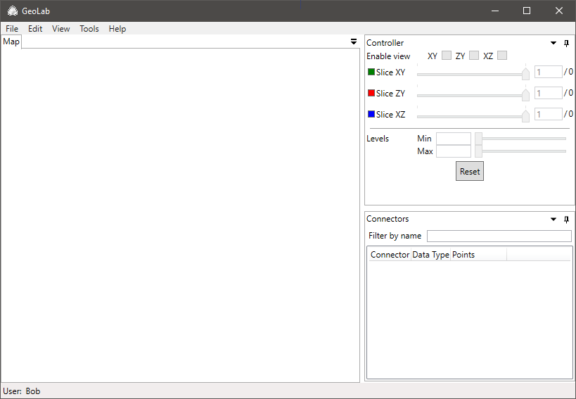
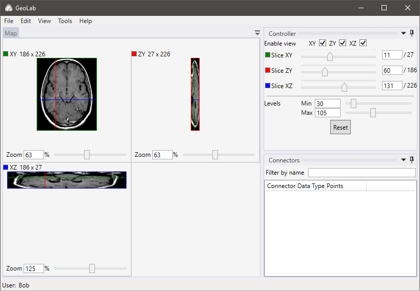
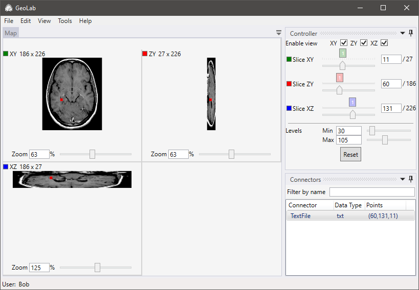
Upon starting the application the main window in Figure 1 is displayed. The main window consists of the menu bar, the container window (containing the Map, Controller and Connectors subwindows) and the status bar (displaying the username). Figure 10 gives more of an idea of what the main window looks like with the 3 Map views displayed and a single connector added.
The section describes the commands in the menu bar of the main window.
The File menu contains the following commands:
| Command | Shortcut | Description |
|---|---|---|
| New | Ctrl+N | Opens a new sample. |
| Open | Ctrl+O | Opens a saved sample file. |
| Save | Ctrl+S | Saves the current sample. |
| Save As | Ctrl+Shift+S | Saves the current sample as a new file. |
| Exit | Ctrl+Q | Closes the application. |
The Edit menu contains the following commands:
| Command | Shortcut | Description |
|---|---|---|
| Add/Change Map | Ctrl+M | Selects a new map file. |
| Add Connector data | Ctrl+D | Adds a new connector. |
| User Preferences | Ctrl+U | Opens a dialog for editing the user preferences. |
The View menu contains the following commands:
| Command | Shortcut | Description |
|---|---|---|
| Axis Colour Coding | F1 | Toggles the coordinate line overlays in the Map view. |
| Attached Data Points | F2 | Toggles the selectable connectors in the Map view. |
| Sample Metadata | F3 | Displays the editable sample metadata. |
The Tools menu contains the following commands:
| Command | Shortcut | Description |
|---|---|---|
| Edit Connectors | Ctrl+E | Toggles the mode where the user can add a connector to the position clicked in the Map view. |
| Create ZY-stack | None | Creates a stack required for viewing the ZY plane. |
| Create XZ-stack | None | Creates a stack required for viewing the XZ plane. |
The Help menu contains the following commands:
| Command | Shortcut | Description |
|---|---|---|
| View Help | F4 | Opens the user manual. |
| About | F5 | Displays the current version, the copyright and the authors of the application. |
Within the main window the user may reposition the subwindows by dragging them from the header and docking them to a new position. A subwindow can also be left undocked as a separate floating window.
The docking tool (see Figure 2) is shown in the main window while dragging a subwindow. A subwindow can be placed above, below, to the left, to the right or in the same place relative to the subwindow below or the container window.

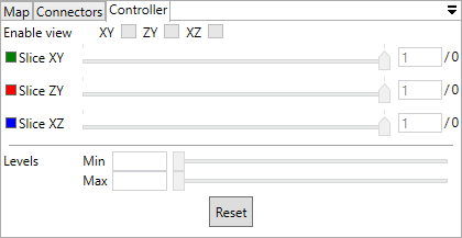
When multiple subwindows share the same space they act as tabs and only one can be viewed at a time (see Figure 3).
In order to view the three dimensional intensity data a map file needs to be added. A map can be read from Edit → Add/Change map. It is possible to change the map file at any time.
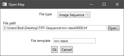
An image sequence is a stack of image files. The read images may be in PNG or TIFF formats. When reading an image
sequence the user has to select a file belonging to the stack. The files should have sequential
names (e.g. image000, image001...) as GeoLab will read them in the natural
order based on naming.
The application will attempt to parse the common name for the images as specified in the field File template. The user may also input the template manually (see Figure 4).
In order to read a multiframe TIFF the user simply needs to select the File type 3D Tiff and then select the file (see Figure 5).
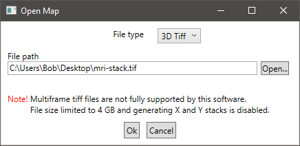
NOTE: The support for multiframe TIFF in GeoLab is limited as follows:
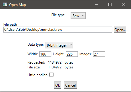
Raw files require the user to input the specific format of the file. These include the data type (8-bit Integer, 16-bit Integer or 32-bit floating point), the horizontal and vertical pixel count of each image, the image count and the endianity. If the dimensions and the data type are set correctly the Requested and File size byte amounts should be equal (see Figure 6). Wrong settings will display the image incorrectly.
By default GeoLab can only display the map file from the original XY plane. In order to enable the XZ and ZY axis views the user must generate XZ and ZY stacks from the original map file.
The stacks can be created from Tools → Create ZY-stack / Create XZ-stack.
The application will attempt to create a folder called XStack or YStack in the location of the
original map file. The user may select this or create another location for the generated stack.
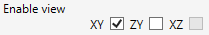
The user cannot cancel the stack generation but they can otherwise continue using the application while the process is underway. The larger the original map file is the longer the stack generation will take. After the stack is generated successfully the Enable view checkbox in the Controller (see Figure 1) will be enabled for the corresponding stack (see Figure 7).
NOTE:
GeoLab allows for viewing the original map and the created stacks slice by slice in each orientation (see Figure 8). The display of the slice view can be enabled or disabled from the Enable view checkboxes of the Controller. The viewed slice of the stack can be changed from the corresponding slider (Slice XY, Slice ZY, Slice XZ) by specifying the number of the slice.
The grayscale of the displayed slices (pixel minimum and maximum values) can be tuned or even inverted from the Controller (see Figure 8). The maximum value is based on the bit depth of the original map. By enabling axis colours from View → Axis Colour Coding an overlay will be added on the images displaying the selected coordinates of the other two axes as lines. The colors used for each axis can be changed in the Edit → User Preferences (see Chapter 11).
NOTE:
GeoLab allows the user attach a file on the computer and metadata related to it with coordinates corresponding to the map. The linked file can be an image, a spreadsheet or plain text. Connectors can also be added before the map has been read and outside the map coordinates.
The supported image formats include bmp, gif, ico, jpg or
jpeg, png, tif or tiff.
The supported spreadsheet formats include csv, xlsx, xlsb, xls.
NOTE:
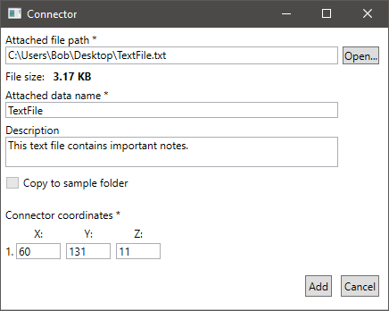
A connector can be added from Edit → Add Connector data (see Figure 9). By default the current coordinates chosen in the sliders are suggested as the position for the new connector. Alternatively the user can select the suggested point by clicking the displayed map image after toggling the Edit Mode from Tools → Edit Connectors.
When the file is selected its name is suggested as the connector name in the Attached data name field. The
user may also give a brief description of the connector which is then saved as connector metadata. The Copy to
sample folder option will copy the file to the location of the saved sample file under the folder
[Sample file name]_AttachedData.
NOTE:
The connectors are listed in the Connectors subwindow (see Figure 10). By right-clicking the connector a context menu will appear with the following options:
| Command | Description |
|---|---|
| Go to | Selects the slices in the Controller that correspond to the connector location (if the coordinates exist on the map). |
| Display | Displays the linked data file in the application. |
| Open File | Opens the linked data file. |
| Open Folder | Opens the file location of the linked data file. |
| Delete selected | Deletes the connector from the sample (doesn't delete the file on the disk). |
| Metadata | Displays the metadata of the connector. |
When adding a new connector the sliders in the Controller are marked with a clickable note with a number of connectors that have been placed on that slice (see Figure 10).
The connectors can also be viewed and selected from the map view by enabling View → Attached Data Points (see Section 4.1). The color of the marking can be customized in the Edit → User Preferences (see Chapter 11).
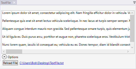
The contents of the linked file can be viewed from the Connectors list by double-clicking the connector (see Figure 10) or selecting Display from the context menu (see Section 8.2). This will open a new subwindow displaying the contents of the file as shown in Figures 11, 12 and 13. If the contents have been edited in another software, the displayed file can be refreshed by opening the Options bottom slide menu and pressing Reload File. If the file has been deleted from the disk the user will be shown an error message when viewing or reloading the file.
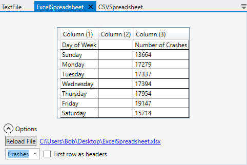
When viewing spreadsheets the rows can be sorted by the value of each column. If the first row of the spreadsheet is dedicated for the headers the checkbox First row as headers in the Options menu should be ticked . When using Excel spreadsheets the sheet of the workbook can also be changed from the Options menu with the drop-down menu (see Figure 12).
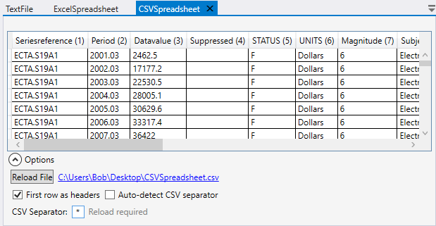
When using the comma separated value (csv) format the application will try to automatically detect the
separator. The user can also select the separator manually. After inputting the separator the spreadsheet needs to
be reloaded (see Figure 13).
The sample can be saved as a json file from File → Save / Save
As. This will save all the links to the map, the created stacks and the linked data relative
to the json file. It is advised that the user stores all the files in a tidy folder structure to make
the transfer of the sample between computers easier. The metadata is also saved to the json file.
NOTE:
GeoLab stores automatically some metadata related to the sample and each connector created. The user is free to add, edit and remove metadata as they please.
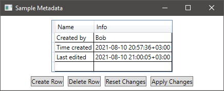
The sample metadata can be accessed from View → Sample Metadata. When saving the sample the application will record the user who created the sample and the datetimes for the creation and latest edit (see Figure 14).
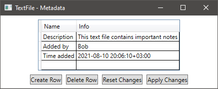
The connector metadata can be accessed by right-clicking the connector from the list in Connectors (see Figure 10) and selecting Metadata. By default the description, the user who added the connector and the datetime for creation are recorded (see Figure 15).
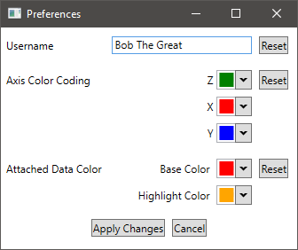
The color coding as well as the username recorded in the metadata can be customized from Edit → User Preferences (see Figure 16). Each value can also be reset to the default value. When resetting the username, the current Windows username will be set.
Axis Color Coding selects the colors for the three main axes used in the Controller and Map. Attached Data Color selects the base and the highlight color for connectors used in the Map (see Figure 10) when the View → Attached Data Points visibility has been toggled.
NOTE:
For issues concerning the use of the application you may contact Jukka Kuva at jukka.kuva@gtk.fi.